Property Variables Most Subject to Endogeneity
Foundations
endogeneity
regression
RCA
The property and market variables most likely to be endogenous in a residential sales model, grouped by cause, with the size and direction of each bias measured in a simulated market whose true price-setting is known; and what that means, under the Residual Constraint Approach, for adjustments, for hypothetical conditions, and for the residual.
Working paper · not peer reviewed
This paper assumes the Residual Constraint Approach (Craytor 2026). The regression takes only measured features. Condition, quality, appeal and the other features the records do not measure are left to the residual: the appraiser ranks the comparable sales by residual, places the subject in that ranking, and other appraisers in the area can check the placement. The CQA score is never used in the primary regression, the one on measured features from which the value conclusion is reached. Where the appraiser rates condition, quality or another of these features, it is only for the purpose of explaining the differences in residuals between properties; the ratings do not enter the regression and do not change the value conclusion.
The definition
This paper uses the definition of the Journal’s entry 009 (Endogeneity), Vol. 1 No. 2, version 1.1.0:
Endogeneity is the condition in which a regressor — a feature the regression uses to explain price — moves with the part of price the model does not explain, so that its estimated coefficient does not recover the causal effect of interest. Its common causes are a feature left out, the price acting back on the feature, the sales being a selected set, and the feature being measured with error.
A coefficient is the number the regression attaches to a feature: in an ordinary linear regression, the change in the estimated price for one more unit of it, the other features held fixed. In MARS the corresponding rate may vary across the feature’s range and with interactions. Two points in the definition carry the rest of this paper.
First, “the part of price the model does not explain” is the structural error, written u: the price minus what the causal relationship says the price should be. Entry 009 (Endogeneity) distinguishes it from the distance between a house’s price and the average price of houses with the same recorded features, which entry 007 (Conditional Expectation) writes ε and which averages zero for every combination of features by construction. A regressor is endogenous when it moves with u; it is exogenous when it does not.
Second, the definition is relative to the causal effect of interest — what the feature does to the price. A coefficient can be a correct description of the sales and still not be that effect. Whether the difference matters depends on the question the coefficient is used to answer.
Endogeneity is therefore not a fixed property of a variable. A variable is endogenous relative to a particular model and a particular causal question: living area can be exogenous for one question and endogenous for another. When this paper calls a variable “subject to endogeneity”, it means that in a residential sales model of the usual kind, read for the usual questions, the variable is often endogenous.
This paper asks which property and market variables are most often in that position, in which direction the resulting error tends to run, and what the appraiser does about it. The test that recurs throughout: a regressor deserves special scrutiny when someone chose its value or measured it using information that also affects price but is not available to the model. The sales as a whole deserve the same scrutiny when what put a house among them — the owner’s decision to sell, or the criteria by which the sales were chosen — is connected to its price.
When it affects the sale price and market value
Endogeneity does not affect every use of a sales model in the same way.
Market value of the property as it is. Market value asks what the property, with the features it actually has, would most probably sell for. For a property valued in its observed state, the principal statistical target is the expected price given the property’s observed features — the conditional expectation of entry 007 (Conditional Expectation). A model can estimate that conditional expectation well even when the coefficients attached to individual features cannot be read as what those features cause. The subject need not closely resemble any single comparable. MARS needs enough data to estimate the value of the subject’s features, and perhaps interactions if specified; where few sales share the subject’s combination of features, the estimate rests on extrapolation and is less reliable.
Endogeneity can affect the value conclusion an appraiser reaches, or the reading of a model’s results, in three situations:
- When a coefficient is read as an adjustment — as what the feature, by itself, is worth — rather than used to predict a price.
- When the value is a counterfactual value — a price for a state of the property that the market has not shown together with this property: value as if remodeled, value subject to completion of an addition, the before-and-after values of a partial taking, any value that disregards the effect of a public project. The sales cannot show these directly.
- When the subject differs from the comparables in the respect that drives the error — for example, a house that reached the top of its market area’s condition by maintenance, priced from comparables that reached it by remodeling.
The market used in this paper
To demonstrate and quantify these errors under known assumptions, rather than discuss them only in the abstract, this paper uses a simulated market of 40,000 houses whose true price-setting is known. It is constructed, not fitted to any real market; its choices are stated in full in the downloadable program endogeneity_sim.py, and a reader can change any of them and rerun it. In outline:
- Location quality, which the sales data do not record, varies from house to house.
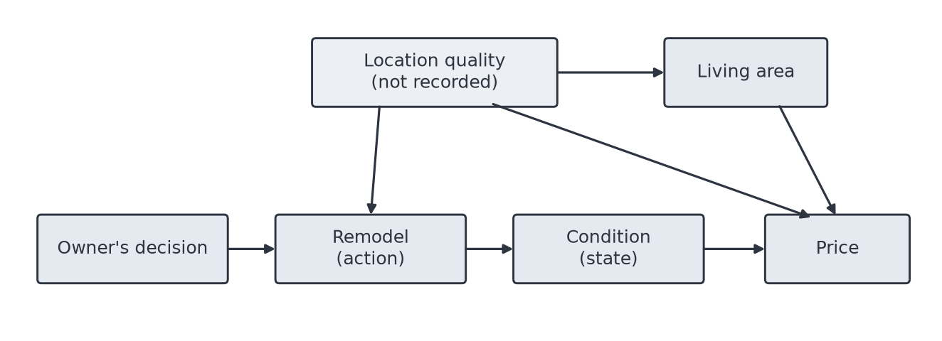
- Remodeling — an action on the property — is more likely where location quality is better and where the house is older: owners remodel where they expect the market to pay. In this market 38% of houses were remodeled.
- Living area is somewhat larger where location quality is better, as additions would be where land value supports them.
- Condition — a state of the property — is scored on the Journal’s scale, 0.00 to 10.00, the score being ten times the share of houses in the market area in worse condition. A remodel raises a house’s condition and does nothing else. (Quality, the other state a remodel can change, is left out of this market to keep each result clear.)
- Price is set by living area ($350 a square foot), location quality, condition ($30,000 a point), age (−$800 a year) and an unexplained part.
So in this market a remodel has no direct effect on price: its whole effect runs through condition. Three causal contrasts follow from it, and the paper names which one it uses each time:
- the effect on the remodeled houses — what the remodels did to the houses that were remodeled: $78,760;
- the effect on the average house — what a remodel would do to a house chosen at random: $78,497;
- the effect on the unremodeled houses — what a remodel would do to the houses that were not remodeled: $78,335.
Every other number below is compared with one of them. Because the market’s price-setting is known, the figures are computed exactly for the 40,000 houses of one draw — they are not estimates from a sample of them, and need no measure of sampling uncertainty (a standard error). Small differences from the parameters that generated the market ($349.5 a square foot against $350, for instance) are chance in that one draw; across ten independent draws they move little — the remodel coefficient of the next section, for instance, ranges from $142,431 to $146,503. They show what each error does in this constructed market; they are not measurements of any real one.
The structure of the market, which the rest of the paper keeps returning to:
In the language of entry 009 (Endogeneity), the remodel is the treatment: the action whose effect is asked about. Price is the outcome. Condition and location quality have roles of their own, a mediator and a confounder, defined under Cause 1 below.
Two kinds of variable: actions and states
The variables of a sales model are not all of one kind, and the difference decides how endogeneity enters.
Actions record that something was done to the property: a recent remodel, recent updates to the kitchen or baths, an addition, a new roof, an accessory dwelling unit. An action is an event — it happened, or it did not, within some period — and it is chosen by the owner.
States describe the property as it is: condition, quality, functional utility, living area, age. A state can be changed by an action — a remodel raises condition and, through finishes and materials, quality — and the market pays for the state the property is in, not for the history of how it got there. Two houses identical in every current state that bears on value should have the same market value, however they reached those states.
In practice, however, those states are only partly observed, and the history of how a house reached them carries information about them. Condition and quality are only partly observed: a score captures what can be seen and judged, not new plumbing and wiring behind the walls, or the workmanship of the work. So a recent remodel or update, even when it adds nothing of its own to the price, remains evidence about the part of the state the scores do not capture, and a model or an appraiser that ignores it ignores real information.
A remodel or update usually tells a buyer something more. Work done under a building permit is inspected at stages, and passed inspections are evidence that the inspected work met the building code’s requirements when it was inspected — wiring, plumbing, structure, fire separation. That evidence is itself part of the property’s state, documented safety and soundness, which a condition score rarely records and a buyer cannot verify on a walk-through. It can reduce a buyer’s uncertainty about concealed components, and so can influence what buyers pay; how much it does in a given market is for the appraisal to establish.
This paper assumes that the local building code and other local regulations were followed, and that every inspection the regulations require was carried out and resulted in approval. Where that is not the case — work done without a required permit, or an inspection not passed — the appraiser has to determine its effect on market value, if any.
The two kinds fail in different ways. An action is often endogenous through the owner’s choice: the houses on which owners act are not a random set (Cause 1 below). A state is often endogenous through its measurement, as recorded living area is (Cause 2), although some states, living area among them, are partly chosen as well. And an action and the states it changes cannot both be read as separate contributions: the state is the channel through which the action reaches the price.
Cause 1: features the owner chose
Actions: remodels, updates, additions
The leading case. The table shows what three ways of reading the sales report for a remodel, against the truth.
| Reading of the sales | Reported | Truth |
|---|---|---|
| Average price of remodeled houses minus average price of the rest | $167,199 | — |
| Remodel coefficient, location not recorded | $144,792 | $78,760 (effect on remodeled houses, through condition) |
| Remodel coefficient, location recorded | $77,999 | ≈ $78,760 (effect on remodeled houses, through condition) |
Constructed market: one draw of 40,000 houses; computed exactly for that draw, not estimated from a sample.
Two lessons follow, and each corresponds to a term from entry 009 (Endogeneity).
The unrecorded location is a confounder. A confounder is a cause of both the feature and the price. Location quality raises the chance of a remodel and raises the price directly. When it is not recorded, the remodel coefficient carries part of its effect: the model reports $144,792 where the remodels did $78,760. Recording location brings the coefficient to $77,999. The difference, $66,793, is the confounding part: it reflects which houses the owners chose to remodel, not anything the work did. (The coefficient with location recorded still differs slightly from the effect on the remodeled houses; the section on counterfactual values returns to that gap.)
Condition is a mediator. A mediator is the channel through which the feature acts on the price: the remodel raises condition, and condition raises the price. For the remodel’s total effect, the channel is therefore not held fixed. Including a variable is the right rule for a confounder and the wrong one for a mediator; neither choice can be made until the effect wanted has been named (entry 009, Endogeneity).
States the owner can choose: living area
Living area is a state, but partly chosen too. Here it is somewhat larger where location quality is better, so when location is not recorded the living-area rate carries part of location’s effect.
| Model | Rate per square foot | Truth |
|---|---|---|
| Location not recorded | $437 | $350 |
| Location recorded | $350 | $350 |
Constructed market: one draw of 40,000 houses; computed exactly for that draw, not estimated from a sample.
The direction of this error depends on how size and location move together in the market at hand. Where larger houses sit on less desirable land, it runs the other way.
Age, through what happened since
The year a house was built is fixed, but which old houses survive, are remodeled or are torn down is not; in some neighborhoods the old houses are the remodeled ones. Age therefore acts partly as a proxy for condition — a measured feature that stands in for one that is not measured — and renovation history, and in the Residual Constraint Approach that is accepted: a later allowance for condition must represent condition not already reflected through age and the other measured features. In the simulated market, where condition falls with age, the age rate with condition left out — as the Residual Constraint Approach leaves it out — is −$2,528 a year, against a true −$800: the age rate has absorbed condition’s effect. Age is also a proxy for the selection behind which houses were remodeled or replaced, and the direction of that part varies from market to market.
Cause 2: features measured with error
Recorded living area differs from the actual living area. The errors in MLS and assessor figures are a mixture of overstatements and understatements, and their sign and size vary from one locality to another. The appraiser in most cases has to rely on MLS data, even though it may be somewhat inaccurate at times. Where the figures are badly wrong, he may have to be very selective in his comparables and check the figures against aerial photographs or by some other method.
Errors of this kind affect the living-area rate, and the rates of features that move with living area — location, lot size, bedroom and bathroom counts — in a direction the sales cannot show. Because the errors vary with the locality, they can make a rate larger or smaller, and more sales do not remove them. Bedroom and bathroom counts move with living area even when the records are exact, which makes it hard to tell how much of the price depends on the number of bathrooms and how much on living area; MARS, which selects the features and the ranges of each feature that carry the price, makes a predictive division between them in the fitted model, although that division need not identify their separate effects.
Cause 3: transaction variables and simultaneity
Simultaneity is the case in which a feature and the price influence each other; a regression of price on such a feature cannot tell how much of their association is the feature’s effect. In sales data it arises chiefly with variables tied to the transaction itself, and these are not all tied to the price in the same way:
- Set before the sale but endogenous: list price. It precedes the final price, but the seller and the broker set it using what they know about the house’s appeal and the market’s likely response — information that also drives the final price.
- Determined together with the price: concessions, seller credits, and some financing terms (others are set by lenders and capital markets largely outside the negotiation).
- Outcomes of the marketing process: days on market. Price and time on the market are products of the same evolving process.
None of these should ordinarily be read as a cause of market value, or used to estimate an adjustment, without an argument for why its relation to price is causal. Some can still help a model predict a price, which is a different use.
School district and neighborhood
Where the data record both the neighborhood and the school district, a model can give the incremental price difference of each, and MARS can do so despite the correlation between them, provided the sales include enough houses in which the two differ; where they seldom differ, the division between them can be unstable. MARS keeps a district term only where the difference improves the model enough. Where a neighborhood contains more than one school district, comparisons within that neighborhood give stronger evidence about the price difference that goes with the district, because many of the neighborhood’s traits are held more nearly constant; they isolate the schools’ own effect only if other price-relevant differences between the district parts of the neighborhood — micro-location, tax jurisdiction, lots — can reasonably be excluded. Elsewhere the district’s figure is a proper location adjustment for a subject in that district, but it cannot be confirmed to be the schools’ effect alone, since traits the model does not record may travel with the district. For the market value of a property as it is, that causes no difficulty, since the subject’s district carries the same traits; it is something for the appraiser to be aware of, and it matters only if the question is about the schools themselves, as when a boundary change moves a house into another district.
Cause 4: which sales are in the data
Selection is the case in which the sales are not a random draw from the houses the conclusion is about, and what put a house among the sales is connected to its price. Owners decide to list before they know what price they will get; but a listing whose offers come in low may be withdrawn or allowed to expire, and it then never appears among the sales. The sold houses are those whose offers were acceptable. The simulated market works this way: a house’s chance of closing rises with how high its offers come in for its features, and 34% of houses sell.
| All houses | Sold houses only | |
|---|---|---|
| Rate per square foot | $349 | $349 |
| Sold houses’ price above the market average for their features | — | $23,181 |
Constructed market: one draw of 40,000 houses; computed exactly for that draw, not estimated from a sample.
In this construction the selection depends only on how high each house’s offers come in for its features, so the rate is unaffected and the whole effect falls on the level: sold houses sit $23,181 above the average for houses with the same features. Where the selection also depends on the features — foreclosures concentrated in some neighborhoods or price ranges, estate sales concentrated among older houses — the rates move as well. Every comparable comes from this selected group.
Market value is what a house can sell for, so sales remain the evidence even for a house that is neither listed nor sold, such as the subject of a refinance appraisal. The question is whether the sales include houses like it. National sales at least include substantial numbers of houses in different states of renovation. In the National Association of Realtors’ 2025 Profile of Home Buyers and Sellers (sales from July 2024 through June 2025), 35% of sellers sold the home as-is, 53% made minor renovations or fixed broken items, and only 12% carried out major renovations. In some areas, especially high-income ones, a larger share of the houses offered for sale have been updated, and the sales may represent fewer of the homes appraised for refinance. Even there, some sold houses are not updated. The difference between them and a subject that is not updated can be adjusted for: in the Residual Constraint Approach, the subject is placed in the ranking among the sales it resembles. A difference becomes harder to support the fewer sales share it, and one that no sale shows needs other evidence.
The variables, summarized
| Variable | Cause | Usual direction of the error in its rate | When it matters |
|---|---|---|---|
| Actions — recent remodel, updates, additions, accessory dwelling unit, pool, solar | Owner’s choice (confounding by unrecorded location, plan, lot) | Up, where owners invest in better houses | Adjustments; counterfactual values |
| Living area | Owner’s choice; record error | Up if size travels with unrecorded location quality; from record error, either way, not shown by the sales | Adjustments |
| Age | What happened since construction (remodel, replacement) | Varies by market | Adjustments |
| List price, days on market, concessions, credits, financing | Set before the sale using price-relevant information (list price); determined with the price (concessions, credits, some financing); outcome of marketing (days on market) | Not interpretable as a cause | Not ordinarily a cause of value or an adjustment; some may help a prediction |
| School district and neighborhood | Unrecorded traits travel with the district | Carried along with the schools’ effect | A matter of awareness; matters only for questions about the schools themselves |
| Sale type and timing | Selection of which houses sell | Level up where owners sell when prices are good; rates move where selection depends on features | All uses; extending a conclusion to unsold houses assumes the sales represent them |
| Position, distance, terrain-fixed view, slope | Physically fixed: not caused by the price, but not necessarily exogenous | — | Can still travel with features the model omits (noise, traffic, prestige); a view across land a neighbor could build on also carries an unrecorded risk of impairment |
Physical fixity rules out the price acting back on such a feature, but not an omitted feature traveling with it: distance to the coast, for instance, can travel with noise, fog or prestige the model does not record. A view across land a neighbor could build on carries something more — an unrecorded risk that the view will be impaired, which a view protected by terrain does not carry — and the two should not be treated as the same feature.
The residual in the Residual Constraint Approach
The ranking and the CQA score
In the Residual Constraint Approach the primary regression takes only the measured features. It is fitted by MARS (multivariate adaptive regression splines, a regression whose rates may change across a feature’s range), using the R package earth. Condition, quality and the other latent features — those the records do not measure — are left out of it on purpose. For each comparable sale in the subject’s market area there are then three figures: its net sale price — the sale price less concessions — the price the regression estimates from its measured features, and the difference between the two, its residual. The comparable sales are ranked by residual, or by residual per square foot of living area, from largest to smallest — the choice is the appraiser’s — and from that ranking each sale’s CQA score (condition, quality and appeal) is formed: 0.00 to 10.00, the percent of the defined market area’s sales with lower residuals, divided by ten. (The residuals exist only for sales; reading the score as a percentile among all the area’s properties assumes the sales are representative of them — the selection question of Cause 4.)
The residual itself is not a measurement of condition, quality and appeal. It contains the value effects of everything the measured-feature model omitted or represented imperfectly, together with error in the model and noise in the transaction:
\[\text{residual}_i \;=\; \underbrace{C_i + Q_i + A_i}_{\text{condition, quality, appeal}} \;+\; \underbrace{L_i + F_i}_{\text{omitted location, other features}} \;+\; \eta_i ,\]
where \(\eta_i\) is model error and negotiation noise. The CQA score orders the sales by the whole residual; it is a residual-placement index used to organize appraisal judgment, not a direct statistical measurement of condition, quality and appeal alone. Attributing that residual to condition, quality, appeal and the other latent features the appraiser judges significant is an appraisal interpretation, constrained by the ranking — not the residual itself.
The ranking is what makes the score checkable. A CQA score of 7.00 makes a definite claim — that seven in ten of the defined market area’s sales have lower residuals — and an auditor, or another appraiser who works in the area, can look at the sales on either side of the subject’s place in the ranking — at their MLS listings and photographs, and from their own knowledge of those houses — and judge whether that placement is reasonable. The appraiser makes the placement by judging all the residual’s latent features together — condition, quality, appeal and the rest — not by scoring each one; the method relies on the comparative judgment of appraisers familiar with the market, and its check is whether another qualified appraiser reviewing the same evidence finds the placement reasonable. Neither a score assigned on an absolute scale nor a coefficient read from a model provides this direct check against neighboring sales in the ranking.
The ranking is also a nonparametric statistic: the CQA score depends only on the order of the residuals, not on their sizes or on any assumed shape of their distribution. It reads the subject’s place directly from the sales’ own residuals, not from a fitted curve, and a few extreme sales move it far less than they would move an average or a fitted coefficient.
Ranking by residual per square foot can be the better measure when the subject is unusually small or large. A small house can carry a much higher degree of quality than a larger one, and in total dollars its residual will still look modest beside the residuals of larger houses. Measured per square foot, its quality shows, and its CQA score is placed accordingly; the same correction keeps a very large house of ordinary quality from ranking high on size alone. Dividing by living area is itself a choice of scale: it suits a market where residuals grow roughly in proportion to living area, and can over- or under-correct where they do not.
What the approach estimates
The CQA score is derived from the difference between the net sale price and the MARS estimated sale price, and it ranks the sales; it never enters the primary regression.
The value conclusion is the regression’s estimate at the subject plus the subject’s residual, the residual being estimated by placing the subject within the ranking. The approach therefore decomposes its valuation estimate into the part predicted from the measured features and a residual assigned from the subject’s place in the ranking; it is not an estimate of how condition impacts value. It does not identify a causal rate for condition, and does not need one.
The subject
The subject is under contract, and its improvements are complete. The approach is applied to an existing property under an executed contract of sale, awaiting its loan and the other conditions of closing. Any remodel or update has been completed; it has already acted on the property’s condition, quality and perhaps other features, and the value sought is the value of the property as it is. The subject’s remodel is therefore not a counterfactual but a fact about the property: valuing the property as it stands does not require identifying the causal effect of remodeling.
That fact still bears on the price. A recent remodel or update raises condition and quality in ways that are not fully observable, so it is evidence for the subject’s place in the ranking; and where the work was done to code with its required inspections passed, it also documents the soundness and safety of what it touched. The market still pays for the state the property is in; the remodel is evidence about that state, much of which lies behind the walls.
Placing the subject
The evidence for the placement: MLS data and photographs. The subject is placed in the ranking by comparing it with the comparables, using the MLS data and, above all, the MLS photographs of each sale. The residuals order the comparables by the part of the net sale price the measured-feature model does not explain; the photographs show what each place in that order looks like — the finishes, the kitchens and baths, the state of repair, the light and the layout of the houses with high residuals, of those in the middle, and of those with low ones. The appraiser places the subject among the comparables whose photographs, and whose listing data, it most resembles in condition, quality and appeal, together with what the inspection of the subject itself shows.
The photographs do three things for the soundness of the placement. They make the ranking interpretable: a sale’s place can be seen to correspond, or not, to what its photographs show, and a sale whose residual its photographs do not explain is a signal to look for an omitted feature or an unusual transaction. They make the placement auditable: the photographs are part of the record, so a reviewer can look at the same evidence the appraiser used rather than take the placement on trust. And the listing photographs were taken to market each house, before its sale price was known, so the evidence itself is not formed with the price in view, even though it is read afterwards. Their limits are known as well: they show what is visible, from angles chosen to show the house at its best, and not what lies behind the walls — which is where the evidence of a recent remodel, and of its passed inspections, adds to them.
A comparable’s residual is everything the measured-feature model did not explain — in the terms of the equation above, its \(C + Q + A\) (including the unobserved part a recent remodel signals), its \(L + F\) (a better micro-location, a better plan) and its \(\eta\) (model error and negotiation noise). Two rules follow for placing the subject, and an auditor can check each one.
- On \(C + Q + A\): place the subject on all observed evidence of its latent state, and on nothing that only travels with that evidence. That the subject was recently remodeled or updated, with its required inspections passed, is evidence of its condition, quality and documented soundness, and belongs in the placement. But if the remodeled comparables sit high in the ranking partly because of their \(L + F\) — location or plan — and the subject does not share those, its placement must not follow them there. The appraiser, unlike the regression, has inspected the subject and has the comparables’ photographs, and can see much of what the model omits.
- On what the model already explained: place the subject on latent value beyond what the measured features carry. If age is partly a proxy for condition, the subject is placed on its condition relative to its age; otherwise the condition counted through age is counted again.
The placement is a judgment, and its check is whether other appraisers who work in the area find it reasonable.
Dividing the residual
Placing the subject fixes its residual as a whole. Dividing a residual among condition, quality, appeal and the other latent features — saying how much of it each contributes — is a separate step, and a harder one. Which latent features to recognize is the appraiser’s judgment: beyond condition, quality and appeal, he may add any he observes to have a significant effect on price — landscaping and yard features, for instance. The techniques available are approximate. Two sales alike in every respect except an update that raised condition from 4.00 to 7.00, for instance, give a price difference for those three points, when such a pair can be found; such pairs are scarce, and the appraiser works with whatever evidence the market area offers. How the residual is divided does not change the value conclusion. The RCA paper proves this (Proof II, p. 36): the total residual adjustment for a comparable equals the subject’s total residual minus the comparable’s, and as long as the components assigned to each property add up to that property’s residual, any reallocation among the components leaves the total — and so the conclusion — unchanged. The division serves to explain the value, not to reach it. An appraiser may rank particular latent features across the market area and give each its own score; such rankings necessarily involve judgment. Under the constraint the contributions assigned to a comparable must sum to its residual, so they do not change the value conclusion; they should still be supportable, because they explain to the report’s user why a comparable’s residual differs from the subject’s, or from the other comparables’. This paper cannot supply the missing evidence. What it offers is a map of where value causation hides, and of the readings of the sales that mislead about it.
Counterfactual values: what the sales cannot show
Counterfactual values arise in assignments other than the contract sale of the previous section: value as if remodeled, subject to completion, before and after a partial taking. For them, ordinary cross-sectional sales — sales from one period, compared across houses rather than over time — do not identify the answer — determine it uniquely, in the sense of entry 010 (Parameter Identification) — when the choice to remodel depends on unrecorded features that also affect price; identifying it takes additional assumptions, additional data, or a research design such as repeat sales: the same house sold before and after the work. The price difference that goes with a remodel in the sales equals what the remodel does plus a part due to which houses were chosen for it. The sales give the sum. The second part cannot be read from them; it has to be assumed, and the value reported as a function of the assumptions.
The confounding part is a product of two quantities
The confounding part is not a free-standing dollar amount. In the linear specification used here, entry 008 (Omitted Variable Bias) gives its exact form, Theil’s formula: the bias in the remodel coefficient from an unrecorded feature is the product of two quantities,
\[\text{confounding part} \;=\; \gamma \cdot \delta ,\]
where \(\gamma\) is how much one unit of the unrecorded feature adds to price under the assumed causal model, and \(\delta\) is how much more of that feature the remodeled houses have than unremodeled houses alike in their recorded features. Both have to be large for the bias to be large: a feature that strongly affects price but is no more common among remodeled houses causes none, and so does one that is far more common among them but does not affect price.
In the simulated market the unrecorded feature is location quality, measured in standard deviations — the typical distance of a house’s location quality from the market’s average. The regression with location recorded puts one standard deviation at $90,904 of price (truth $90,000), and remodeled houses have 0.73 standard deviations more of it than unremodeled houses alike in living area and age. Their product, $66,793, is exactly the excess of the remodel coefficient ($144,792) over the coefficient with location recorded ($77,999).
Two assumptions, reported as a grid
For a counterfactual value the appraiser therefore assumes two things about the confounding part, each of which can be argued from knowledge of the market: how much the unrecorded qualities that attract remodeling — micro-location, plan, lot — add to price (\(\gamma\)), and how much more of them the houses that get remodeled tend to have (\(\delta\)). The report shows the conclusion over a range of both. Where possible, the ranges are judged against observed features of known importance: could the omitted qualities matter as much to price, or travel as strongly with remodeling, as recorded location does? For an unremodeled house in the simulated market, the gain from remodeling, by assumption:
| More unrecorded quality among remodeled houses (δ, standard deviations) | γ = $30,000 | γ = $60,000 | γ = $90,000 | γ = $120,000 |
|---|---|---|---|---|
| 0.25 | $137,292 | $129,792 | $122,292 | $114,792 |
| 0.50 | $129,792 | $114,792 | $99,792 | $84,792 |
| 0.75 | $122,292 | $99,792 | $77,292 | $54,792 |
| 1.00 | $114,792 | $84,792 | $54,792 | $24,792 |
Gain from remodeling = observed coefficient − γ·δ. γ: price added by one standard deviation of unrecorded quality. Constructed market: one draw of 40,000 houses; computed exactly for that draw, not estimated from a sample.
The true average gain for the unremodeled houses of this market — the effect on the unremodeled houses — is $78,335, near the cell for \(\delta\) = 0.75 and \(\gamma\) = $90,000, close to the true values. Two cautions remain. First, the product accounts only for the confounding feature. Any difference between the condition gain of the houses that were remodeled and of those that were not is a further, separate gap between the coefficient and the effect wanted, which the product does not capture and the sales cannot separate; in this market it is small (the coefficient with location recorded, $77,999, against an effect on the unremodeled houses of $78,335). Second, nothing in the sales identifies \(\gamma\) or \(\delta\). The grid does not give the answer an aura of identification it does not have; it shows the reader how the conclusion depends on assumptions that are stated.
This follows the general logic of sensitivity analysis for unmeasured confounding (Rosenbaum 2002; Cinelli and Hazlett 2020): identify what the observed data do not determine, vary it over a defensible range, and report how the conclusion changes. The grid is a simplified practitioner heuristic, not that formal procedure. Cinelli and Hazlett express the two quantities as partial \(R^2\) values — each the share of the treatment’s, and of the price’s, remaining variation that the omitted confounder would explain — derive bounds on the bias from them that hold for any number of omitted variables combined, and calibrate the bounds against observed features (an omitted confounder “as strong as location”, for instance). The dollar form here writes the same product, \(\gamma \cdot \delta\), for a single omitted feature acting linearly, in units an appraiser can argue about; it sets the two quantities by judgment, without that calibration, and its grid is a range of stated assumptions, not a bound. Where a study needs a defensible bound rather than a stated assumption, the formal procedure is the one to use. It has the same structure as the Residual Constraint Approach: what the data cannot divide is assigned by the appraiser under stated assumptions, and the conclusion is reported conditioned on them. Only the features the counterfactual changes need such assumptions; the others stay at the subject’s actual values.
The seller’s question
A seller deciding which updates to make before listing asks the counterfactual question directly: for this house, which update raises the price by more than it costs? The easy answer can mislead. The price difference updated houses show in the sales overstates the gain where updates go disproportionately to houses with favorable unrecorded features, as in the simulated market; where they go to distressed houses, as investors’ renovations may, it can understate it.
What an update yields also depends on where the house starts. In the simulated market, the same remodel yields on average:
| Condition the house would have without the remodel | Average gain |
|---|---|
| below 3.00 | $79,227 |
| 3.00 to 7.00 | $94,103 |
| 7.00 and above | $41,490 |
Constructed market: one draw of 40,000 houses; computed exactly for that draw, not estimated from a sample.
The physical improvement is the same in every row, and so is the price of a condition point ($30,000); what differs is how many points the same improvement adds. Because the score is a rank — ten times the share of the market area’s houses in worse condition — what matters is how many houses the improvement carries the house past. The scores themselves are spread evenly by construction (30% of houses below 3.00, 40% from 3.00 to 7.00, 30% above); the houses’ underlying condition is not, and the same improvement passes more houses where it is most bunched together, in the middle, than in either tail, while near the top the ceiling of 10.00 leaves little room. In points:
| Condition the house would have without the remodel | Condition points added |
|---|---|
| below 3.00 | 2.64 |
| 3.00 to 7.00 | 3.14 |
| 7.00 and above | 1.38 |
Constructed market: one draw of 40,000 houses; computed exactly for that draw, not estimated from a sample. Starting condition is scored against the market as it stands.
The two tables rest on different things. The points come from the scale: on any rank scale the same improvement adds fewer points where few houses stand, and none past the ceiling. The dollars come from the constructed market as well: it pays the same $30,000 for every point, so the smaller dollar gain at the top only repeats the smaller number of points. A real market need not pay the same for every point; buyers may pay more for the step from 9.00 to 10.00 than for the step from 5.00 to 6.00, and in such a market the dollar gain at the top could match or exceed the gain in the middle. Whether they do is a question about the market area, not about the scale, and nothing in these tables answers it. The Residual Constraint Approach does not assume an answer: it reads the residual at the subject’s place in the ranking from the comparables there, so whatever the market pays at the top is in the residuals of the sales at the top.
For a seller, the practical question is therefore how many of the market area’s houses the update would carry the subject past, and what the market area’s buyers pay at the place it would reach. Work beyond the level that buyers in the market area pay for is not fully recovered in the sale price.
Updates that change measured features — an added bathroom, space that becomes living area — move the model’s prediction by the rate at the subject’s position, subject to the endogeneity of living area above. Updates that change latent features — paint, flooring, a kitchen refresh, landscaping — move the subject up the residual ranking, and the estimate is where it would land, judged on the features the update changes while holding fixed what it does not: location, plan, light, lot.
Work done to code, with its required inspections passed, carries one further return: passed inspections are evidence of code compliance for the inspected work, and may reduce buyers’ and lenders’ uncertainty.
Particularly strong observational evidence comes from repeat sales — the same house sold before and after its renovation — in which the house’s own unchanging, unrecorded qualities cancel — provided the market change over the interval, and any other change to the house or its surroundings, can be accounted for. One caution remains: houses renovated by investors are chosen for their upside, so the gains observed on them may overstate what a renovation would yield on a house chosen at random.
What a report should state
- The question each coefficient is used to answer: a prediction, an adjustment, or a counterfactual value.
- For each adjustment, whether the feature is one listed above, and the likely direction of its error.
- For a counterfactual value, the two assumptions behind the confounding part — how much the unrecorded qualities add to price, and how much more of them the selected houses have — the reasoning for their ranges, and the value over those ranges.
- In the Residual Constraint Approach, the basis on which the subject was placed among the comparables’ residuals — the MLS data and photographs of the subject and of the comparables on either side of its place.
Limits of this paper
The paper assumes the Residual Constraint Approach. The simulated market is linear (it pays the same for every square foot and every condition point), has one confounder, and is constructed to show each cause clearly; real markets have several confounders at once, and MARS models rates that change across a feature’s range. The underlying mechanisms carry over, but with several confounders and interactions their effects need not separate cleanly feature by feature, and the sizes do not carry over: the figures above show the direction and mechanism of each error, not its size in any real market. The program is published so that its assumptions can be changed and the consequences seen. One interaction deserves a specific warning. A MARS model fitted where remodeling is concentrated above some age or below some condition could place a knot — a point where a rate changes — there, and encode the association created by selection in the fitted shape of the rate, where it is harder to see than in a single coefficient. The published program is linear; to examine this, make the price function nonlinear in age or condition and fit it with earth. The simulation demonstrates how each kind of error arises, not how common it is: whether a particular variable is endogenous in a particular market, and the size and direction of the resulting bias, have to be investigated in the market and the data being analyzed.
References
- The Valuation Engineer Journal, Foundations, Vol. 1 No. 2 (2026): entry 007 (Conditional Expectation), entry 008 (Omitted Variable Bias), entry 009 (Endogeneity), entry 010 (Parameter Identification).
- Craytor, W. B. (2026). Residual Constraint Approach (RCA): Framework & Protocol. The Valuation Engineer, 1(1). https://doi.org/10.67330/kgebxf46
- Cinelli, C., & Hazlett, C. (2020). Making Sense of Sensitivity: Extending Omitted Variable Bias. Journal of the Royal Statistical Society, Series B, 82(1), 39–67.
- Theil, H. (1957). Specification Errors and the Estimation of Economic Relationships. Revue de l’Institut International de Statistique, 25(1/3), 41–51.
- National Association of Realtors (2025). 2025 Profile of Home Buyers and Sellers. Chicago: National Association of Realtors.
- Rosenbaum, P. R. (2002). Observational Studies (2nd ed.). Springer.
Appendix: the logic as a Prolog program
The program below states the logic of this paper as facts and rules, so that a reader can query it: which variables are endogenous and by which cause, when that matters, whether a variable is included for the effect wanted, the confounding part \(\gamma \cdot \delta\) and its grid, the CQA score from a list of residuals, the placement rules, and Proof II of the RCA paper — that dividing a residual differently leaves the adjustment unchanged. It builds on the vocabulary of entry 009 (Endogeneity) without loading it, and runs under Trealla (the Journal’s official Prolog), SWI-Prolog and Scryer Prolog. Its self-test runs each time this page is built; the result is printed after the listing. The file can be downloaded from the link at the top of the page.
% SPDX-License-Identifier: AGPL-3.0-or-later
% Copyright (C) 2026 William Bert Craytor. Published by Valuation Engineer
% Research Labs (Pacific Vista Net). This program is free software: you can
% redistribute it and/or modify it under the terms of the GNU Affero General
% Public License as published by the Free Software Foundation, either version 3
% of the License, or (at your option) any later version. It is distributed
% WITHOUT ANY WARRANTY, without even the implied warranty of MERCHANTABILITY or
% FITNESS FOR A PARTICULAR PURPOSE; see
% <https://www.gnu.org/licenses/agpl-3.0.html>.

%% property-variables-endogeneity.pl
%%
%% Prolog companion to the working paper
%%   "Property Variables Most Subject to Endogeneity" (Research Labs, 2026)
%%   Author:  Bert Craytor
%%   Version: 1.0.0 (draft)
%%
%% It states the logic of the paper as facts and rules, so that a reader can
%% query it. It builds on the vocabulary of Foundations entry
%% 009 (Endogeneity), Vol. 1 No. 2, version 1.1.0, without loading it: this
%% file runs on its own. It runs under Trealla (the Journal's official
%% Prolog), SWI-Prolog and Scryer Prolog.
%%
%% Try:
%%   ?- run_tests.
%%   ?- often_endogenous_via(living_area, Cause).
%%   ?- matters_for(days_on_market, Use).
%%   ?- confounding_part(0.75, 90000, X).
%%   ?- cqa_score(12000, [-30000,-8000,0,5000,15000,22000], S).

:- use_module(library(lists)).
:- dynamic(moves_with_structural_error/3).   % filled in for a given model

% ---------------------------------------------------------------------------
% 1. The method assumed
% ---------------------------------------------------------------------------

method_assumed(residual_constraint_approach).

% Features the records measure, and those they do not (latent).
measured(living_area).
measured(age).
measured(lot_size).
measured(bedrooms).
measured(bathrooms).

latent(condition).
latent(quality).
latent(appeal).
latent(unrecorded_location).
latent(other_unmeasured_features).

% Only measured features are eligible for the primary regression, the one
% from which the value conclusion is reached; MARS selects among them. The
% CQA score and the appraiser's ratings of latent features never enter it.
eligible_for_primary_regression(F) :- measured(F).

% What the appraiser's ratings of latent features are for.
purpose_of_latent_ratings(explain_residual_differences_between_properties).
affects_value_conclusion(latent_ratings, no).

% The residual of a comparable sale and its components.
residual_definition(residual = net_sale_price - primary_regression_estimate).
net_sale_price_definition(net_sale_price = sale_price - concessions).
residual_component(cqa,       [condition, quality, appeal]).
residual_component(omitted,   [unrecorded_location, other_unmeasured_features]).
residual_component(eta,       [model_error, negotiation_noise]).

% ---------------------------------------------------------------------------
% 2. The definition (entry 009, Endogeneity) and the scrutiny test
% ---------------------------------------------------------------------------

% A regressor is endogenous, relative to a model and a causal question,
% when it moves with the structural error u.
endogenous(Regressor, Model, Question) :-
    moves_with_structural_error(Regressor, Model, Question).

% The test that recurs through the paper. A regressor deserves scrutiny
% when someone chose its value or measured it using price-relevant
% information the model does not have. Selection is a property of the
% sales as a whole, not of one regressor: they deserve the same scrutiny
% when what put a house among them is connected to its price.
scrutiny_reason(regressor, chosen).
scrutiny_reason(regressor, measured).
scrutiny_reason(sales_as_a_whole, owners_decision_to_sell).
scrutiny_reason(sales_as_a_whole, criteria_for_choosing_the_sales).

% ---------------------------------------------------------------------------
% 3. When endogeneity affects the sale price and market value
% ---------------------------------------------------------------------------

affects_value(reading_a_coefficient_as_an_adjustment).
affects_value(counterfactual_value).
affects_value(subject_unlike_comparables_in_the_driving_respect).

% Market value of the property as it is: the target is the conditional
% expectation (entry 007, Conditional Expectation), which a model can
% estimate well even when its coefficients are not causal effects.
unaffected_target(market_value_as_is, conditional_expectation,
                  provided(subject_features_covered_by_comparables)).

% ---------------------------------------------------------------------------
% 4. Actions and states
% ---------------------------------------------------------------------------

variable_kind(recent_remodel,           action).
variable_kind(recent_updates,           action).
variable_kind(addition,                 action).
variable_kind(accessory_dwelling_unit,  action).
variable_kind(pool,                     action).
variable_kind(solar,                    action).
variable_kind(condition,                state).
variable_kind(quality,                  state).
variable_kind(functional_utility,       state).
variable_kind(living_area,              state).
variable_kind(age,                      state).

changes(recent_remodel, condition).
changes(recent_remodel, quality).
changes(recent_updates, condition).
changes(recent_updates, quality).

% How each kind usually becomes endogenous.
common_route(action, owner_choice).
common_route(state,  measurement).
common_route(state,  owner_choice).        % living area is partly chosen

% An action is evidence about the part of the state the ratings miss, and
% work done to code with inspections passed documents safety and soundness.
evidence_about(Action, State) :- changes(Action, State).
documents(Action, safety_and_soundness) :-
    variable_kind(Action, action),
    assumed(code_followed), assumed(required_inspections_approved).

assumed(code_followed).
assumed(required_inspections_approved).

% ---------------------------------------------------------------------------
% 5. Roles and the inclusion rule (entry 009, Endogeneity)
% ---------------------------------------------------------------------------

role(remodel,          treatment).
role(condition,        mediator).
role(location_quality, confounder).
role(price,            outcome).

% Whether to include a variable depends on the effect wanted.
include_rule(confounder, _AnyEffect,   yes).
include_rule(mediator,   total_effect, no).
include_rule(mediator,   direct_effect, yes).

include_variable(V, Effect, Answer) :-
    role(V, Role), include_rule(Role, Effect, Answer).

% ---------------------------------------------------------------------------
% 6. The variables, by cause (the paper's summary table)
% ---------------------------------------------------------------------------

often_endogenous_via(recent_remodel,       owner_choice).
often_endogenous_via(recent_updates,       owner_choice).
often_endogenous_via(addition,             owner_choice).
often_endogenous_via(accessory_dwelling_unit, owner_choice).
often_endogenous_via(pool,                 owner_choice).
often_endogenous_via(solar,                owner_choice).
often_endogenous_via(living_area,          owner_choice).
often_endogenous_via(living_area,          record_error).
often_endogenous_via(age,                  what_happened_since_construction).
often_endogenous_via(list_price,           set_with_price_relevant_information).
often_endogenous_via(concessions,          determined_with_price).
often_endogenous_via(seller_credits,       determined_with_price).
often_endogenous_via(financing_terms,      determined_with_price).  % some
often_endogenous_via(days_on_market,       outcome_of_marketing).
often_endogenous_via(sale_type_and_timing, selection).

% School district and neighborhood: a proper location adjustment for the
% market value as is; unrecorded traits travel with the district, which
% matters only for questions about the schools themselves.
awareness(school_district, unrecorded_traits_travel_with_it).
matters_only_for(school_district, questions_about_the_schools_themselves).

% Physically fixed: not caused by the price, but not necessarily exogenous;
% such a feature can still travel with features the model omits. A view
% across land a neighbor could build on also carries an unrecorded risk of
% impairment, and is not the same feature as a view protected by terrain.
physically_fixed(position).
physically_fixed(distance).
physically_fixed(terrain_fixed_view).
physically_fixed(slope).
carries_unrecorded_risk(view_across_buildable_land, impairment).

usual_direction(recent_remodel, owner_choice,
                up_where_owners_invest_in_better_houses).
usual_direction(living_area, owner_choice,
                up_if_size_travels_with_unrecorded_location).
usual_direction(living_area, record_error,
                either_way_not_shown_by_the_sales).
usual_direction(age, what_happened_since_construction, varies_by_market).
usual_direction(sale_type_and_timing, selection,
                level_up_rates_move_if_selection_depends_on_features).

matters_for(V, adjustment) :-
    often_endogenous_via(V, C), first_cause(V, C), C \== selection,
    \+ transaction_variable(V).
matters_for(V, counterfactual_value) :-
    variable_kind(V, action), often_endogenous_via(V, owner_choice).
matters_for(V, not_a_cause_of_value) :- transaction_variable(V).
matters_for(sale_type_and_timing, every_use).

first_cause(V, C) :- often_endogenous_via(V, C1), !, C = C1.


transaction_variable(list_price).
transaction_variable(concessions).
transaction_variable(seller_credits).
transaction_variable(financing_terms).
transaction_variable(days_on_market).

% ---------------------------------------------------------------------------
% 7. Measurement error
% ---------------------------------------------------------------------------

% Recorded living area: MLS and assessor errors vary in sign and size by
% locality, so their effect on the living-area rate, and on the rates of
% features that move with living area, cannot be read from the sales.
record_error_effect(living_area, direction_not_shown_by_the_sales).
reaches_rates_of(living_area, [location, lot_size, bedrooms, bathrooms]).

% Record error is not removed by adding comparables.
removed_by_more_comparables(record_error, no).

% ---------------------------------------------------------------------------
% 8. The confounding part (Theil's formula, entry 008, Omitted Variable
%    Bias; exact in the linear specification)
% ---------------------------------------------------------------------------

% Gamma: price added by one unit of the unrecorded feature.
% Delta: how much more of it the remodeled houses have.
confounding_part(Delta, Gamma, Part) :- Part is Gamma * Delta.

% Gain from remodeling, given the observed coefficient and the assumptions.
gain(Coefficient, Delta, Gamma, Gain) :-
    confounding_part(Delta, Gamma, Part),
    Gain is Coefficient - Part.

% The paper's grid (observed coefficient from the simulated market).
observed_remodel_coefficient(144792).
grid_delta(0.25). grid_delta(0.50). grid_delta(0.75). grid_delta(1.00).
grid_gamma(30000). grid_gamma(60000). grid_gamma(90000). grid_gamma(120000).

grid_cell(Delta, Gamma, Gain) :-
    observed_remodel_coefficient(B),
    grid_delta(Delta), grid_gamma(Gamma),
    G0 is B - Gamma * Delta, Gain is round(G0).

% The grid is a practitioner heuristic: a range of stated assumptions for
% one omitted feature acting linearly, not a formal bound
% (Cinelli and Hazlett 2020 give the formal bounds).
grid_is(stated_assumptions).
grid_is_not(formal_bound).

% ---------------------------------------------------------------------------
% 9. The CQA score and the placement of the subject
% ---------------------------------------------------------------------------

ranking_basis(residual).
ranking_basis(residual_per_square_foot).   % the appraiser chooses

% CQA score: percent of the market area's sales with lower residuals, / 10.
cqa_score(SubjectResidual, Residuals, Score) :-
    count_lower(Residuals, SubjectResidual, Lower),
    length(Residuals, N), N > 0,
    Score is 10 * Lower / N.

count_lower([], _, 0).
count_lower([R|Rs], X, C) :-
    count_lower(Rs, X, C0),
    ( R < X -> C is C0 + 1 ; C = C0 ).

placement_evidence(mls_data).
placement_evidence(mls_photographs).

placement_rule(1, cqa,
    place_on_all_observed_evidence_of_latent_state_not_on_what_travels_with_it).
placement_rule(2, measured,
    place_on_latent_value_beyond_what_the_measured_features_carry).

placement_check(other_appraisers_in_the_area_find_it_reasonable).

% ---------------------------------------------------------------------------
% 10. Dividing the residual does not change the conclusion (RCA Proof II)
% ---------------------------------------------------------------------------

% A division of a residual is a list of contributions that sum to it.
valid_division(Residual, Parts) :- sum(Parts, S), S =:= Residual.

% Total residual adjustment for a comparable: subject's residual minus the
% comparable's, whatever the division.
residual_adjustment(SubjectParts, CompParts, Adjustment) :-
    sum(SubjectParts, S), sum(CompParts, C),
    Adjustment is S - C.

sum([], 0).
sum([X|Xs], S) :- sum(Xs, S0), S is S0 + X.

% ---------------------------------------------------------------------------
% 11. What a report should state
% ---------------------------------------------------------------------------

report_item(1, question_each_coefficient_answers).
report_item(2,
    for_each_adjustment_whether_listed_and_likely_direction_of_error).
report_item(3, counterfactual_value_two_assumptions_ranges_and_value_over_them).
report_item(4, basis_of_subject_placement_mls_data_and_photographs).

% ---------------------------------------------------------------------------
% Self-test
% ---------------------------------------------------------------------------

test(rca_assumed,           method_assumed(residual_constraint_approach)).
test(cqa_not_in_regression, \+ eligible_for_primary_regression(cqa_score)).
test(latent_not_in_regression,
     \+ (latent(F), eligible_for_primary_regression(F))).
test(ratings_explanatory,   affects_value_conclusion(latent_ratings, no)).
test(remodel_is_action,     variable_kind(recent_remodel, action)).
test(condition_is_state,    variable_kind(condition, state)).
test(include_confounder,
     include_variable(location_quality, total_effect, yes)).
test(exclude_mediator,      include_variable(condition, total_effect, no)).
test(living_area_two_causes,
     ( often_endogenous_via(living_area, owner_choice),
       often_endogenous_via(living_area, record_error) )).
test(record_error_direction,
     record_error_effect(living_area, direction_not_shown_by_the_sales)).
test(no_cancelling,         removed_by_more_comparables(record_error, no)).
test(theil_product,
     ( confounding_part(0.735, 90904, P), abs(P - 66814.44) < 0.01 )).
test(grid_cell,             grid_cell(0.75, 90000, 77292)).
test(cqa_score,
     ( cqa_score(12000, [-30000,-8000,0,5000,15000,22000], S),
       abs(S - 6.6667) < 0.001 )).
test(proof_ii,
     ( valid_division(40000, [25000, 10000, 5000]),
       valid_division(40000, [10000, 20000, 10000]),
       valid_division(15000, [9000, 6000]),
       valid_division(15000, [3000, 12000]),
       residual_adjustment([25000, 10000, 5000], [9000, 6000], A1),
       residual_adjustment([10000, 20000, 10000], [3000, 12000], A2),
       A1 =:= A2 )).
test(two_rules,
     ( placement_rule(2, measured, _), \+ placement_rule(3, _, _) )).
test(one_answer_per_use,
     ( findall(U, matters_for(living_area, U), Us), Us == [adjustment] )).
test(pool_is_action,        matters_for(pool, counterfactual_value)).
test(financing_terms,       transaction_variable(financing_terms)).
test(not_a_cause,           matters_for(days_on_market, not_a_cause_of_value)).
test(district_awareness,
     matters_only_for(school_district, questions_about_the_schools_themselves)).
test(physically_fixed,      physically_fixed(terrain_fixed_view)).
test(view_risk,
     carries_unrecorded_risk(view_across_buildable_land, impairment)).

run_tests :-
    findall(Name, test(Name, _), Names),
    run_each(Names, 0, Failed),
    length(Names, N),
    Passed is N - Failed,
    write(Passed), write(' of '), write(N), write(' tests passed.'), nl,
    Failed =:= 0.

run_each([], F, F).
run_each([Name|Ns], F0, F) :-
    test(Name, Goal),
    ( call(Goal) -> F1 = F0
    ; write('FAIL: '), write(Name), nl, F1 is F0 + 1 ),
    run_each(Ns, F1, F).
?- run_tests
23 of 23 tests passed.
Quiz
Fifteen questions on endogeneity, each with one best answer. The answers are printed upside down at the bottom of the page.
Under the definition of entry 009 (Endogeneity), a regressor is endogenous when it:
- is measured with any error at all.
- moves with the part of price the model does not explain, so that its coefficient does not recover the causal effect of interest.
- moves with another feature in the model.
- has a large standard error.
Is living area an endogenous variable?
- Always: it is chosen by owners.
- Never: it is measured in square feet.
- Only when it is taken from public records.
- It depends on the model and the question: a variable is endogenous relative to a particular model and a particular causal question.
In which of these does endogeneity not ordinarily affect the value conclusion?
- A coefficient is read as an adjustment — as what the feature, by itself, is worth.
- A value as if remodeled.
- The expected price of a subject in its observed state, from comparables that cover its features.
- A subject that reached the top of its market area’s condition by maintenance, priced from comparables that reached it by remodeling.
According to the paper’s recurring test, a regressor deserves special scrutiny when:
- its coefficient is larger than expected.
- someone chose its value or measured it using information that also affects price but is not available to the model.
- it has many missing values.
- it was added to the model last.
Actions (a recent remodel, an addition) and states (condition, quality) often become endogenous in different ways. How?
- An action often through the owner’s choice; a state often through its measurement.
- An action often through its measurement; a state often through the owner’s choice.
- Both chiefly through simultaneity.
- Neither can be endogenous.
A feature the model leaves out biases the coefficient of a feature it includes only when the omitted feature:
- is measured with error.
- affects price.
- moves with the included feature.
- both affects price and moves with the included feature: the bias is the product of the two (Theil’s formula, entry 008, Omitted Variable Bias).
In the simulated market, larger houses stand in better locations, and location quality is not recorded. The living-area rate is $437 a square foot, against a true $350. Why?
- The living-area rate carries part of the effect of the unrecorded location.
- Recorded living area differs from the actual area.
- The market pays more for large houses.
- Chance in the simulated draw.
In the simulated market condition falls with age, and the model leaves condition out. The age rate is −$2,528 a year, against a true −$800. Why?
- Old houses sell in a different market.
- Age acts partly as a proxy for condition, and its rate absorbs condition’s effect.
- Age is measured with error.
- The price acts back on age.
Recorded living area runs high in some localities of the market area and low in others. Its effect on the living-area rate:
- always makes the rate smaller.
- disappears with enough sales.
- cannot be read from the sales: it may make the rate larger or smaller, and it also reaches the rates of features that move with living area.
- affects only the intercept.
A model records both the neighborhood and the school district, and MARS keeps a price difference for some of the districts. What does that tell the appraiser?
- Every district in the area affects price by the same amount.
- The district terms cannot be used, because district and neighborhood are correlated.
- MARS found that keeping a district term improved the model enough to survive its selection procedure.
- The schools are of higher quality in those districts.
Days on market, list price, concessions and seller credits should ordinarily not be read as causes of value or used to estimate an adjustment, because:
- they are not recorded in the MLS.
- they are always small.
- they are set with price-relevant information, determined together with the price, or outcomes of the same marketing process.
- USPAP prohibits their use.
In the definition of entry 009 (Endogeneity), “the part of price the model does not explain” is:
- the difference between a house’s price and the average price of houses with the same recorded features.
- the price minus what the causal relationship says the price should be — the structural error.
- the sampling error of the regression.
- the concessions in the sale.
Why can a model whose coefficients are not causal effects still estimate the market value of a property as it is?
- Because MARS removes endogeneity.
- It cannot; every coefficient must be causal.
- Because endogeneity only affects counterfactual values in court.
- Because the target is the expected price given the property’s observed features (entry 007, Conditional Expectation). The subject need not closely resemble any single comparable, but the sales must cover its features well enough; where few sales share its combination of features, the estimate rests on extrapolation and is less reliable.
Two houses have the same recorded view: one is protected by terrain, the other looks across a neighboring vacant lot on which someone could build. Which statement is correct?
- The second view carries an unrecorded risk of impairment, so the two should not be treated as the same feature.
- Both views are exogenous (opposite of endogenous) because they are physically fixed.
- The two views are identical for valuation.
- A view is a transaction variable.
Why are repeat sales of the same house particularly strong evidence?
- Because the second price is always higher.
- Because they need no adjustment for market change.
- Because the house’s own unchanging, unrecorded qualities cancel, provided the market change over the interval, and any other change to the house or its surroundings, can be accounted for.
- Because they come from a selected set.
Answers.
1 b — “The definition”, entry 009 (Endogeneity).
2 d — “The definition”.
3 c — “When it affects the sale price and market value”.
4 b — “The definition”, the recurring test.
5 a — “Two kinds of variable: actions and states”.
6 d — “Counterfactual values”; entry 008 (Omitted Variable Bias).
7 a — Cause 1, “States the owner can choose: living area”.
8 b — Cause 1, “Age, through what happened since”.
9 c — Cause 2, features measured with error.
10 c — “School district and neighborhood”: keeping a term is MARS’s model selection, not a significance test.
11 c — Cause 3, transaction variables.
12 b — “The definition”; (a) is the error of entry 007 (Conditional Expectation), which averages zero by construction.
13 d — “When it affects the sale price and market value”.
14 a — “The variables, summarized”: physical fixity does not make a feature exogenous.
15 c — “The seller’s question”, repeat sales.